Introduction
I decided to write a series of tutorials about Elasticsearch aggregations. In this first post of the series, we are going to deal with the bucket aggregations that allow us to implement faceted navigation.
What is Elasticsearch
Elasticsearch is an opensource JSON-based search engine that allows us to search indexed data quickly and with options that are not provided by classic data stores.
Elasticsearch is a distributed, RESTful search and analytics engine capable of solving a growing number of use cases. As the heart of the Elastic Stack, it centrally stores your data so you can discover the expected and uncover the unexpected. – official Elasticsearch product page
What is Kibana
Kibana is a tool mainly allowing visualization of Elasticsearch data. We will use Kibana because it also provides a very convenient way for writing and executing queries (with autocomplete).
Kibana lets you visualize your Elasticsearch data and navigate the Elastic Stack, so you can do anything from learning why you’re getting paged at 2:00 a.m. to understanding the impact rain might have on your quarterly numbers. – official Kibana product page
What are Elasticsearch bucket aggregations
Before familiarizing myself with the term aggregations in the Elasticsearch world, what I was actually trying to learn was how to implement the widely known feature of facets for my indexed data.
Chances are that you know about facets, you have seen it in many sites. They are usually placed as a sidebar in search results landing pages and they are rendered as links or checkboxes that act as filters to help you narrow the results based on their properties.
A section of Elasticsearch’s aggregations framework named bucket aggregations provides the functionality we need to implement a faceted navigation.
Bucket aggregations don’t calculate metrics over fields like the metrics aggregations do, but instead, they create buckets of documents. Each bucket is associated with a criterion (depending on the aggregation type) which determines whether or not a document in the current context “falls” into it. In other words, the buckets effectively define document sets. In addition to the buckets themselves, the bucket aggregations also compute and return the number of documents that “fell into” each bucket. – official elasticsearch bucket aggregations reference
Prerequisites
In order to be able to execute the tutorial’s commands and queries, you must first:
Install Elasticsearch (duh)
Providing instructions for installing Elasticsearch is out of scope. I recommend visiting the product’s related documenation site. After the installation, just make sure to start the service if it’s not started. You can check that with
curl http://localhost:9200
It should give something like:
{
  "name" : "blabla",
  "cluster_name" : "elasticsearch",
  "cluster_uuid" : "blabla",
  "version" : {
    "number" : "6.4.2",
    "build_flavor" : "default",
    "build_type" : "deb",
    "build_hash" : "04711c2",
    "build_date" : "2018-09-26T13:34:09.098244Z",
    "build_snapshot" : false,
    "lucene_version" : "7.4.0",
    "minimum_wire_compatibility_version" : "5.6.0",
    "minimum_index_compatibility_version" : "5.0.0"
  },
  "tagline" : "You Know, for Search"
}
As you can see, we will use Elasticsearch version 6.4.2 in this tutorial.
Install Kibana
I recommend following the official instructions for installing kibana at your machine’s OS. I followed this guide for installing the product via a repository in Ubuntu.
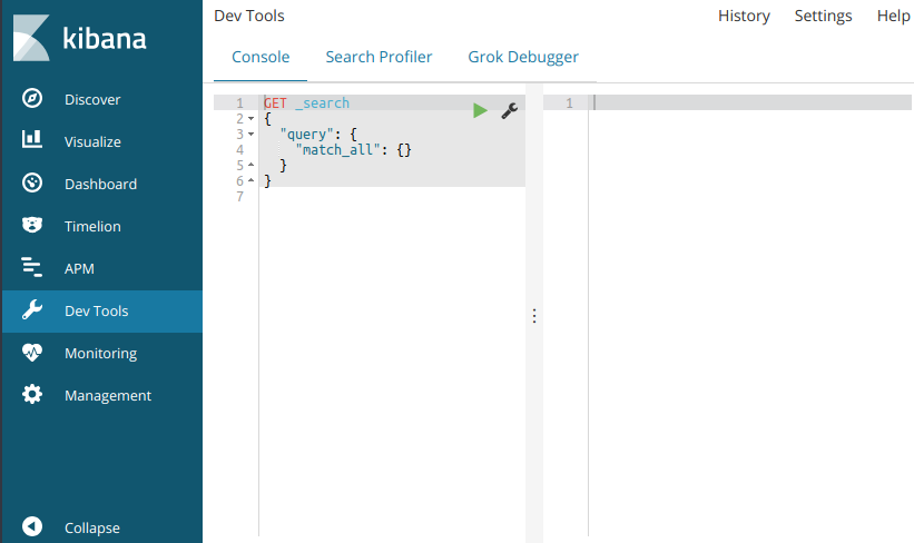
Start the kibana service and navigate to its home page at http://localhost:5601. We will heavily use the Dev Tools which is a powerful console talking to the Elasticsearch engine.
What is it going to be covered
We are going to deal with:
- Terms aggregations
- Sub-aggregations
- Nested and reverse nested aggregations
- Global aggregations
Don’t be afraid, everything will become very clear once we start playing with the data.
Hands on
Let the fun begin.
The model
Suppose that we want to implement a web application for city pet registrations. We will define the following entities:
- City office: a city pet registration office
- city: the city in which the office is located
- office type: the type of the office (central, district)
- Citizen: a citizen with registered pets
- occupation: the occupation of the citizen
- age: the age of the citizen
- Pet: a citizen’s pet
- kind: the kind of the pet (cat, dog etc)
- name: the name of the pet
- age: the age of the pet
Our entities relations are:
- One city office has many citizens
- One citizen has many registered pets
Prepare the data
Before starting explaining the aggregations, we first have to create the index to store our data and then we have to feed this index with sample data.
Create the index
Navigate to Kibana’s Dev Tools page and execute the following request:
PUT city_offices
{
  "settings": {
    "number_of_shards": 1
  },
  "mappings": {
    "_doc": {
      "properties": {
        "city": {
          "type": "keyword"
        },
        "office_type": {
          "type": "keyword"
        },
        "citizens": {
          "type": "nested",
          "properties": {
            "occupation": {
              "type": "keyword"
            },
            "age": {
              "type": "integer"
            },
            "pets": {
              "type": "nested",
              "properties": {
                "kind": {
                  "type": "keyword"
                  },
                "name": {
                  "type": "keyword"
                },
                "age": {
                  "type": "integer"
                }
              }
            }
          }
        }
      }
    }
  }
}
In the output section, you should see:
{
  "acknowledged": true,
  "shards_acknowledged": true,
  "index": "city_offices"
}
We created an index with name city_offices with the aforementioned properties.
Important note: we chose to define the entity relations as nested objects. Why?
The nested type is a specialized version of the object datatype that allows arrays of objects to be indexed in a way that they can be queried independently of each other … Lucene has no concept of inner objects, so Elasticsearch flattens object hierarchies into a simple list of field names and values – official elasticsearch nested datatype reference
I will explain this with an example.
Suppose we had a city office with two citizens. One 35 year old Dentist and one 30 year old Developer. If we used the object datatype, Elasticsearch would merge all sub-properties of the entity relation resulting to something like this:
{
  "citizens": {
    "occupation": ["Dentist", "Developer"],
    "age": ["35", "30"]
  }
}
Thus, if we wanted to search the index for offices that have a Dentist citizen with age 30, this document would fulfill the criteria even though the Dentist is 35 years old.
Mapping the relation as nested overcomes this problem since
Internally, nested objects index each object in the array as a separate hidden document, meaning that each nested object can be queried independently of the others – official elasticsearch nested datatype reference
Feed sample data
I have created some sample data with random cities, occupations, pet names etc. You can find it at this tutorial’s GitHub repo.
Download the file sample-data.json and from within the download folder execute:
curl -s -H "Content-Type: application/x-ndjson" -XPOST http://localhost:9200/_bulk --data-binary "@sample-data.json"; echo
Note: The data were generated with this ruby script. You can alter it as you please and execute it to produce your desired sample data json file.
That’s it. Aggregations time.
Aggregation request format
All aggregation queries are embedded in search requests.
GET <index_name>/_search
{
  "query": { ... },
  "aggs": {
    "<aggregation name>": {
      "<aggregation type>": { <aggregation properties> }
    }
  }
}
where:
- aggregation name: is the name we give to our aggregation. This is required in order to be able to parse the search response afterwards and locate the specific aggregation results (you will understand this better after we execute the first aggregation request).
- aggregation type: is the type of the aggregation we want to execute. You can browse all available aggregations provided by Elasticsearch here.
- aggregation properties: are the available properties specific to the aggregation type.
Terms aggregations
We will use the Terms aggregation in order to find out how many different values our documents have in a specific field.
Navigate to Kibana’s Dev Tools section and in the console (left section of the page) type the following:
GET city_offices/_search
{
  "aggs": {
    "cities": {
      "terms": { "field": "city" }
    }
  }
}
Following the syntax described in the Aggregation request format section above
- we are searching in the
city_officesindex - we are requesting an aggregation of type
terms - we specify that we are interested in the different values of the field
city
Now execute the request by pressing the play link that you should be seeing given that the query you typed is focused.
Voila!
{
  "took": 2,
  "timed_out": false,
  "_shards": {
    "total": 1,
    "successful": 1,
    "skipped": 0,
    "failed": 0
  },
  "hits": {
    "total": 113,
    "max_score": 1,
    "hits": [
      {
        ...
      }
    ]
  },
  "aggregations": {
    "cities": {
      "doc_count_error_upper_bound": 0,
      "sum_other_doc_count": 37,
      "buckets": [
        {
          "key": "Amsterdam",
          "doc_count": 8
        },
        {
          "key": "London",
          "doc_count": 8
        },
        {
          "key": "Oslo",
          "doc_count": 8
        },
        {
          "key": "Paris",
          "doc_count": 8
        },
        {
          "key": "San Francisco",
          "doc_count": 8
        },
        {
          "key": "Tokyo",
          "doc_count": 8
        },
        {
          "key": "Athens",
          "doc_count": 7
        },
        {
          "key": "Barcelona",
          "doc_count": 7
        },
        {
          "key": "Chicago",
          "doc_count": 7
        },
        {
          "key": "Madrid",
          "doc_count": 7
        }
      ]
    }
  }
}
Since we are executing a search request, the response contains the hits attribute with all the results matching our query (in this case all documents since we didn’t add a query). It also contains though another attribute named aggregations and that’s where our aggregation results fall under.
Inside the aggregations you can see our cities aggregation and that’s why it is required to name the aggregations you define.
Before explaining the weird sum_other_doc_count 37 value, let’s first examine the buckets.
There’s our different values for the city field of the city offices. “Human reading” the values, we have 8 offices in Amsterdam, London, Oslo, Paris, San Francisco and Tokyo, 7 offices in Athens, Barcelona, Chicago and Madrid.
The total of these offices is 76 but the search response says we have 113. Let’s subtract the bucket’s office total from the actual total offices: (113 - 76 = 37) == sum_other_doc_count. That’s right. Explanation: the aggregation we defined has another property named size which has a default value of 10. Since we didn’t define another value, Elasticsearch limited the buckets to the top 10 different city values based on their occurrences in the index. 37 are the documents whose cities are not listed in the buckets and NOT the number of the unlisted cities.
Let’s change the size to 50 (hoping that we don’t have offices in more than 50 cities).
GET city_offices/_search
{
  "size": 0,
  "aggs": {
    "cities": {
      "terms": {
        "field": "city",
        "size": 50
      }
    }
  }
}
Hint: In addition to defining the aggregation’s size, I also set in the top level query the size to 0 so that I can browse the response faster since the hits attribute will be empty.
Execute again.
{
  "took": 1,
  "timed_out": false,
  "_shards": {
    "total": 1,
    "successful": 1,
    "skipped": 0,
    "failed": 0
  },
  "hits": {
    "total": 113,
    "max_score": 0,
    "hits": []
  },
  "aggregations": {
    "cities": {
      "doc_count_error_upper_bound": 0,
      "sum_other_doc_count": 0,
      "buckets": [
        {
          "key": "Amsterdam",
          "doc_count": 8
        },
        {
          "key": "London",
          "doc_count": 8
        },
        {
          "key": "Oslo",
          "doc_count": 8
        },
        {
          "key": "Paris",
          "doc_count": 8
        },
        {
          "key": "San Francisco",
          "doc_count": 8
        },
        {
          "key": "Tokyo",
          "doc_count": 8
        },
        {
          "key": "Athens",
          "doc_count": 7
        },
        {
          "key": "Barcelona",
          "doc_count": 7
        },
        {
          "key": "Chicago",
          "doc_count": 7
        },
        {
          "key": "Madrid",
          "doc_count": 7
        },
        {
          "key": "New York",
          "doc_count": 7
        },
        {
          "key": "Warsaw",
          "doc_count": 7
        },
        {
          "key": "Berlin",
          "doc_count": 6
        },
        {
          "key": "Budapest",
          "doc_count": 6
        },
        {
          "key": "Melbourne",
          "doc_count": 6
        },
        {
          "key": "Prague",
          "doc_count": 5
        }
      ]
    }
  }
}
Perfect. The previously missed cities are now fetched and the sum_other_doc_count’s 0 value confirms that we haven’t left any document outside the aggregation.
Let’s add another aggregation for the offices, this time for their type.
GET city_offices/_search
{
  "size": 0,
  "aggs": {
    "cities": {
      "terms": {
        "field": "city",
        "size": 50
      }
    },
    "office_types": {
      "terms": {
        "field": "office_type"
      }
    }
  }
}
We defined another terms aggregation named office_types and kept the default bucket size since we know that we don’t have more than 10 distinct office types.
{
  "took": 1,
  "timed_out": false,
  "_shards": {
    "total": 1,
    "successful": 1,
    "skipped": 0,
    "failed": 0
  },
  "hits": {
    "total": 113,
    "max_score": 0,
    "hits": []
  },
  "aggregations": {
    "cities": {
      "doc_count_error_upper_bound": 0,
      "sum_other_doc_count": 0,
      "buckets": [
        ...
      ]
    },
    "office_types": {
      "doc_count_error_upper_bound": 0,
      "sum_other_doc_count": 0,
      "buckets": [
        {
          "key": "primary",
          "doc_count": 57
        },
        {
          "key": "secondary",
          "doc_count": 56
        }
      ]
    }
  }
}
So, we have 57 primary and 56 secondary offices and 0 offices left outside the aggregation’s buckets.
For example, if we want to see how many different office types are in Athens, we can specify the appropriate search query without altering the aggregations’ one.
GET city_offices/_search
{
  "size": 0,
  "query": {
    "term": {
      "city": {
        "value": "Athens"
      }
    }
  },
  "aggs": {
    "cities": {
      "terms": {
        "field": "city",
        "size": 50
      }
    },
    "office_types": {
      "terms": {
        "field": "office_type",
        "size": 10
      }
    }
  }
}
Execute and…
{
  "took": 2,
  "timed_out": false,
  "_shards": {
    "total": 1,
    "successful": 1,
    "skipped": 0,
    "failed": 0
  },
  "hits": {
    "total": 7,
    "max_score": 0,
    "hits": []
  },
  "aggregations": {
    "cities": {
      "doc_count_error_upper_bound": 0,
      "sum_other_doc_count": 0,
      "buckets": [
        {
          "key": "Athens",
          "doc_count": 7
        }
      ]
    },
    "office_types": {
      "doc_count_error_upper_bound": 0,
      "sum_other_doc_count": 0,
      "buckets": [
        {
          "key": "secondary",
          "doc_count": 5
        },
        {
          "key": "primary",
          "doc_count": 2
        }
      ]
    }
  }
}
We have 5 secondary and 2 primary offices in Athens.
What if we wanted to have this information for all cities without having to limit the search’s results? In other words, what if we wanted to present the facets like this:
Read the next section.
Sub-bucket aggregations
The Terms aggregations (and other type of aggregations) allow the definition of sub-aggregations. The sub-aggregations are executed in the documents belonging to the bucket of the parent aggregation. It’s like asking: Give me the different cities. Ok, now give me for each one how many office types it has.
The syntax of sub-aggregations is pretty straight forward.
GET <index_name>/_search
{
  "query": { ... },
  "aggs": {
    "<aggregation name>": {
      "<aggregation type>": { <aggregation properties> },
      "aggs": {
        "<sub-aggregation name>": {
          "<sub-aggregation type>": { <sub-aggregation properties> }
        }
      }
    }
  }
}
Applying the above in our case, all we have to do is to define the search request as follows:
GET city_offices/_search
{
  "size": 0,
  "aggs": {
    "cities": {
      "terms": {
        "field": "city",
        "size": 50
      },
      "aggs": {
        "office_types": {
          "terms": {
            "field": "office_type"
          }
        }
      }
    },
    "office_types": {
      "terms": {
        "field": "office_type",
        "size": 10
      }
    }
  }
}
The response:
{
  "took": 12,
  "timed_out": false,
  "_shards": {
    "total": 1,
    "successful": 1,
    "skipped": 0,
    "failed": 0
  },
  "hits": {
    "total": 113,
    "max_score": 0,
    "hits": []
  },
  "aggregations": {
    "cities": {
      "doc_count_error_upper_bound": 0,
      "sum_other_doc_count": 0,
      "buckets": [
        {
          "key": "Amsterdam",
          "doc_count": 8,
          "office_types": {
            "doc_count_error_upper_bound": 0,
            "sum_other_doc_count": 0,
            "buckets": [
              {
                "key": "primary",
                "doc_count": 4
              },
              {
                "key": "secondary",
                "doc_count": 4
              }
            ]
          }
        },
        {
          "key": "London",
          "doc_count": 8,
          "office_types": {
            "doc_count_error_upper_bound": 0,
            "sum_other_doc_count": 0,
            "buckets": [
              {
                "key": "primary",
                "doc_count": 6
              },
              {
                "key": "secondary",
                "doc_count": 2
              }
            ]
          }
        },
        {
          "key": "Oslo",
          "doc_count": 8,
          "office_types": {
            "doc_count_error_upper_bound": 0,
            "sum_other_doc_count": 0,
            "buckets": [
              {
                "key": "primary",
                "doc_count": 4
              },
              {
                "key": "secondary",
                "doc_count": 4
              }
            ]
          }
        },
        {
          "key": "Paris",
          "doc_count": 8,
          "office_types": {
            "doc_count_error_upper_bound": 0,
            "sum_other_doc_count": 0,
            "buckets": [
              {
                "key": "primary",
                "doc_count": 4
              },
              {
                "key": "secondary",
                "doc_count": 4
              }
            ]
          }
        },
        {
          "key": "San Francisco",
          "doc_count": 8,
          "office_types": {
            "doc_count_error_upper_bound": 0,
            "sum_other_doc_count": 0,
            "buckets": [
              {
                "key": "primary",
                "doc_count": 4
              },
              {
                "key": "secondary",
                "doc_count": 4
              }
            ]
          }
        },
        ...
      ]
    },
    "office_types": {
      "doc_count_error_upper_bound": 0,
      "sum_other_doc_count": 0,
      "buckets": [
        {
          "key": "primary",
          "doc_count": 57
        },
        {
          "key": "secondary",
          "doc_count": 56
        }
      ]
    }
  }
}
If we wanted to retrieve even more sub-results for another property of the city offices (for example building type), we could add a sub-aggregation inside the already defined office_types sub-aggregation of the cities aggregation.
Awesome. Time to play with the pets.
Nested aggregations
As previously mentioned, we defined the city office’s relations as nested objects. In order to perform aggregations on these relations we have to follow another approach, the Nested aggregations.
A special single bucket aggregation that enables aggregating nested documents. – official Elasticsearch Nested Aggregation reference
Syntax:
GET <index_name>/_search
{

  "aggs" : {
    "<aggregation-name>" : {
      "nested" : {
        "path" : "<nested-object-path>"
      },
      "aggs" : {
        "<nested-aggregation-name>": {
          "<aggregation-type>" : { <aggregation-properties> }
        }
      }
    }
  }
}
where nested-object-path is the navigation path of the desired object in the root document. For example, if we want aggregations for the citizens we will set this property to citizens. If we wanted aggregations for the pets, we will set this property to citizens.pets.
Let’s see how we can breakdown the number of citizens per occupation.
GET city_offices/_search
{
  "size": 0,
  "aggs": {
    "citizens": {
      "nested": {
        "path": "citizens"
      },
      "aggs": {
        "occupations": {
          "terms": {
            "field": "citizens.occupation",
            "size": 50
          }
        }
      }
    }
  }
}
The response:
{
  "took": 0,
  "timed_out": false,
  "_shards": {
    "total": 1,
    "successful": 1,
    "skipped": 0,
    "failed": 0
  },
  "hits": {
    "total": 113,
    "max_score": 0,
    "hits": []
  },
  "aggregations": {
    "citizens": {
      "doc_count": 3966,
      "occupations": {
        "doc_count_error_upper_bound": 0,
        "sum_other_doc_count": 0,
        "buckets": [
          {
            "key": "Hairdresser",
            "doc_count": 243
          },
          {
            "key": "Microbiologist",
            "doc_count": 241
          },
          {
            "key": "Farmer",
            "doc_count": 234
          },
          {
            "key": "Marketing Manager",
            "doc_count": 231
          },
          {
            "key": "Clinical Laboratory Technician",
            "doc_count": 230
          },
          {
            "key": "Librarian",
            "doc_count": 230
          },
          {
            "key": "Editor",
            "doc_count": 229
          },
          ...
        ]
      }
    }
  }
}
So, there are 3966 citizens that have registered their pets to our city offices of which 243 are Hairdressers, 241 are Microbiologists etc.
Ok good, but what if wanted to see in how many offices are these citizens registered. In other words, how many offices have Marketing Managers? How many offices have Librarians?
Reverse nested aggregations
We have to use another type of aggregation, named Reverse nested aggregation.
A special single bucket aggregation that enables aggregating on parent docs from nested documents. Effectively this aggregation can break out of the nested block structure and link to other nested structures or the root document, which allows nesting other aggregations that aren’t part of the nested object in a nested aggregation.
The reverse_nested aggregation must be defined inside a nested aggregation. –official Elasticsearch Reverse nested aggregation reference
Even though it might sound complicated, it’s not. And playing around with the data is the best way for understanding the provided functionality of any feature.
Syntax:
GET <index_name>/_search
{

  "aggs" : {
    "<aggregation-name>" : {
      "nested" : {
        "path" : "<nested-object-path>"
      },
      "aggs" : {
        "<nested-aggregation-name>": {
          "<aggregation-type>" : { <aggregation-properties> },
          "aggs": {
            "in_offices": {
              "reverse_nested": { <reverse-nested-options> }
            }
          }
        }
      }
    }
  }
}
As you can see, the reverse nested aggregation is always defined as a sub-aggregation inside a nested aggregation.
Time to see in how many offices each occupation is spread.
GET city_offices/_search
{
  "size": 0,
  "aggs": {
    "citizens": {
      "nested": {
        "path": "citizens"
      },
      "aggs": {
        "occupations": {
          "terms": {
            "field": "citizens.occupation",
            "size": 50
          },
          "aggs": {
            "in_offices": {
              "reverse_nested": {}
            }
          }
        }
      }
    }
  }
}
{
  "took": 0,
  "timed_out": false,
  "_shards": {
    "total": 1,
    "successful": 1,
    "skipped": 0,
    "failed": 0
  },
  "hits": {
    "total": 113,
    "max_score": 0,
    "hits": []
  },
  "aggregations": {
    "citizens": {
      "doc_count": 3966,
      "occupations": {
        "doc_count_error_upper_bound": 0,
        "sum_other_doc_count": 0,
        "buckets": [
          {
            "key": "Hairdresser",
            "doc_count": 243,
            "in_offices": {
              "doc_count": 98
            }
          },
          {
            "key": "Microbiologist",
            "doc_count": 241,
            "in_offices": {
              "doc_count": 98
            }
          },
          {
            "key": "Farmer",
            "doc_count": 234,
            "in_offices": {
              "doc_count": 99
            }
          },
          {
            "key": "Marketing Manager",
            "doc_count": 231,
            "in_offices": {
              "doc_count": 91
            }
          },
          {
            "key": "Clinical Laboratory Technician",
            "doc_count": 230,
            "in_offices": {
              "doc_count": 98
            }
          },
          {
            "key": "Librarian",
            "doc_count": 230,
            "in_offices": {
              "doc_count": 98
            }
          },
          ...
        ]
      }
    }
  }
}
Translating the response, we have 243 Hairdressers registered in 98 offices, 241 Microbiologists registered in 98 offices, 234 Farmers registered in 99 offices etc.
The reverse nested aggregation accepts a single option named path. This options defines how many steps backwards in the document hierarchy we want Elasticsearch to go to calculate the aggregations. In our case, since citizens is the immediate relation of the city office type we had to leave it undefined implying that we want the aggregations of the occupations to be calculated against the root object a.k.a. the offices. Confused? Don’t worry, it will become clear after playing around with the pets. Now.
How many pets per kind are registered per citizen?
GET city_offices/_search
{
  "size": 0,
  "aggs": {
    "citizens": {
      "nested": {
        "path": "citizens.pets"
      },
      "aggs": {
        "kinds": {
          "terms": {
            "field": "citizens.pets.kind",
            "size": 10
          },
          "aggs": {
            "per_citizen": {
              "reverse_nested": {}
            }
          }
        }
      }
    }
  }
}
Note that we didn’t define the path option and
{
  "took": 1,
  "timed_out": false,
  "_shards": {
    "total": 1,
    "successful": 1,
    "skipped": 0,
    "failed": 0
  },
  "hits": {
    "total": 113,
    "max_score": 0,
    "hits": []
  },
  "aggregations": {
    "citizens": {
      "doc_count": 11845,
      "kinds": {
        "doc_count_error_upper_bound": 0,
        "sum_other_doc_count": 0,
        "buckets": [
          {
            "key": "Dog",
            "doc_count": 2421,
            "per_citizen": {
              "doc_count": 113
            }
          },
          {
            "key": "Hamster",
            "doc_count": 2403,
            "per_citizen": {
              "doc_count": 113
            }
          },
          {
            "key": "Cat",
            "doc_count": 2380,
            "per_citizen": {
              "doc_count": 113
            }
          },
          {
            "key": "Bird",
            "doc_count": 2330,
            "per_citizen": {
              "doc_count": 113
            }
          },
          {
            "key": "Rabbit",
            "doc_count": 2311,
            "per_citizen": {
              "doc_count": 113
            }
          }
        ]
      }
    }
  }
}
So, there are 2421 registered dogs, 2403 registered hamsters, 2380 registered cats etc. The per_citizen bucket info though doesn’t seem right. Does the 113 number ring a bell? Exactly, that’s how many offices we have. Since we didn’t define the path in the reverse nested aggregation, Elasticsearch calculated the count of root documents (a.k.a. the offices) that have each pet kind registered. Let’s fix that.
GET city_offices/_search
{
  "size": 0,
  "aggs": {
    "citizens": {
      "nested": {
        "path": "citizens.pets"
      },
      "aggs": {
        "kinds": {
          "terms": {
            "field": "citizens.pets.kind",
            "size": 10
          },
          "aggs": {
            "per_citizen": {
              "reverse_nested": {
                "path": "citizens"
              }
            }
          }
        }
      }
    }
  }
}
There it is:
{
  "took": 0,
  "timed_out": false,
  "_shards": {
    "total": 1,
    "successful": 1,
    "skipped": 0,
    "failed": 0
  },
  "hits": {
    "total": 113,
    "max_score": 0,
    "hits": []
  },
  "aggregations": {
    "citizens": {
      "doc_count": 11845,
      "kinds": {
        "doc_count_error_upper_bound": 0,
        "sum_other_doc_count": 0,
        "buckets": [
          {
            "key": "Dog",
            "doc_count": 2421,
            "per_citizen": {
              "doc_count": 1864
            }
          },
          {
            "key": "Hamster",
            "doc_count": 2403,
            "per_citizen": {
              "doc_count": 1852
            }
          },
          {
            "key": "Cat",
            "doc_count": 2380,
            "per_citizen": {
              "doc_count": 1823
            }
          },
          {
            "key": "Bird",
            "doc_count": 2330,
            "per_citizen": {
              "doc_count": 1803
            }
          },
          {
            "key": "Rabbit",
            "doc_count": 2311,
            "per_citizen": {
              "doc_count": 1800
            }
          }
        ]
      }
    }
  }
}
There are 2421 dogs registered by 1864 citizens, 2403 hamsters registered by 1852 citizens, 2380 cats registered by 1823 citizens etc.
Note: Each citizen has more than one pets which can be of different kind that’s why the per_citizen sum of doc_count is way bigger than our citizens.
Before moving on to the last type of aggregations, let’s execute a more advanced nested query answering to the questions:
For each city, how many kind of pets are registered per citizen occupation and in how many offices?
Breaking down the question, we have to think like this:
- Since we want results per city, we are going to add a Terms aggregation on the field
city - Since we want to have results per citizen occupation, we are going to add a Terms sub-aggregation on the field
occupation.- Since the citizen is a nested object, the aggregation of the previous item has to be a sub-aggregation of a Nested aggregation on the path
citizen
- Since the citizen is a nested object, the aggregation of the previous item has to be a sub-aggregation of a Nested aggregation on the path
- Since we want to have results per pet kind, we are going to add a Terms sub-aggregation on the field
kind.- Since the pet is a nested object, the aggregation of the previous item has to be a sub-aggregation of a Nested aggregation on the path
citizen.pets
- Since the pet is a nested object, the aggregation of the previous item has to be a sub-aggregation of a Nested aggregation on the path
GET city_offices/_search
{
  "size": 0,
  "aggs": {
    "cities": {
      "terms": {
        "field": "city",
        "size": 50
      },
      "aggs": {
        "citizens": {
          "nested": {
            "path": "citizens"
          },
          "aggs": {
            "occupations": {
              "terms": {
                "field": "citizens.occupation",
                "size": 50
              },
              "aggs": {
                "pets": {
                  "nested": {
                    "path": "citizens.pets"
                  },
                  "aggs": {
                    "kinds": {
                      "terms": {
                        "field": "citizens.pets.kind",
                        "size": 10
                      },
                      "aggs": {
                        "per_occupation": {
                          "reverse_nested": {
                            "path": "citizens"
                          }
                        },
                        "per_office": {
                          "reverse_nested": {}
                        }
                      }
                    }
                  }
                }
              }
            }
          }
        }
      }
    }
  }
}
{
  "took": 17,
  "timed_out": false,
  "_shards": {
    "total": 1,
    "successful": 1,
    "skipped": 0,
    "failed": 0
  },
  "hits": {
    "total": 113,
    "max_score": 0,
    "hits": []
  },
  "aggregations": {
    "cities": {
      "doc_count_error_upper_bound": 0,
      "sum_other_doc_count": 0,
      "buckets": [
        {
          "key": "Amsterdam",
          "doc_count": 8,
          "citizens": {
            "doc_count": 230,
            "occupations": {
              "doc_count_error_upper_bound": 0,
              "sum_other_doc_count": 0,
              "buckets": [
                {
                  "key": "Dancer",
                  "doc_count": 19,
                  "pets": {
                    "doc_count": 49,
                    "kinds": {
                      "doc_count_error_upper_bound": 0,
                      "sum_other_doc_count": 0,
                      "buckets": [
                        {
                          "key": "Cat",
                          "doc_count": 13,
                          "per_office": {
                            "doc_count": 5
                          },
                          "per_occupation": {
                            "doc_count": 9
                          }
                        },
                        {
                          "key": "Rabbit",
                          "doc_count": 11,
                          "per_office": {
                            "doc_count": 5
                          },
                          "per_occupation": {
                            "doc_count": 10
                          }
                        },
                        {
                          "key": "Bird",
                          "doc_count": 9,
                          "per_office": {
                            "doc_count": 5
                          },
                          "per_occupation": {
                            "doc_count": 7
                          }
                        },
                        {
                          "key": "Dog",
                          "doc_count": 8,
                          "per_office": {
                            "doc_count": 5
                          },
                          "per_occupation": {
                            "doc_count": 7
                          }
                        },
                        {
                          "key": "Hamster",
                          "doc_count": 8,
                          "per_office": {
                            "doc_count": 3
                          },
                          "per_occupation": {
                            "doc_count": 7
                          }
                        }
                      ]
                    }
                  }
                },
                ...
              ]
            }
          }
        },
        ...
        ]
      }
    }
  }
}
“Human” reading the response, in Amsterdam there are 8 offices with 230 citizens that have registered pets of which:
- 19 are Dancers that have registered a total of 49 pets of which
- 13 are cats registered by 9 dancers in 5 offices
- 11 are rabbits registered by 10 dancers in 5 offices
- …
- 8 are hamsters registered by 7 dancers in 3 offices
- I stop this now because I got dizzy
Global aggregations
I will end this tutorial with something easier. Global aggregations.
Defines a single bucket of all the documents within the search execution context. This context is defined by the indices and the document types you’re searching on, but is not influenced by the search query itself. – official Elasticsearch Global aggregation reference
To better explain this, let’s re-think of query:
GET city_offices/_search
{
  "size": 0,
  "aggs": {
    "cities": {
      "terms": {
        "field": "city",
        "size": 50
      },
      "aggs": {
        "office_types": {
          "terms": {
            "field": "office_type"
          }
        }
      }
    },
    "office_types": {
      "terms": {
        "field": "office_type",
        "size": 10
      }
    }
  }
}
which would help us build this form:
When we render such a form, what is the expected behavior once he/she clicks on a checkbox, for example London? Well, we expect the aggregations to be re-applied to the search results that were narrowed by the clicked facet. So the request will become:
GET city_offices/_search
{
  "size": 0,
  "query": {
    "term": {
      "city": {
        "value": "London"
      }
    }
  },
  "aggs": {
    "cities": {
      "terms": {
        "field": "city",
        "size": 50
      },
      "aggs": {
        "office_types": {
          "terms": {
            "field": "office_type",
            "size": 10
          }
        }
      }
    }
  }
}
and the response:
{
  "took": 0,
  "timed_out": false,
  "_shards": {
    "total": 1,
    "successful": 1,
    "skipped": 0,
    "failed": 0
  },
  "hits": {
    "total": 8,
    "max_score": 0,
    "hits": []
  },
  "aggregations": {
    "cities": {
      "doc_count_error_upper_bound": 0,
      "sum_other_doc_count": 0,
      "buckets": [
        {
          "key": "London",
          "doc_count": 8,
          "office_types": {
            "doc_count_error_upper_bound": 0,
            "sum_other_doc_count": 0,
            "buckets": [
              {
                "key": "primary",
                "doc_count": 6
              },
              {
                "key": "secondary",
                "doc_count": 2
              }
            ]
          }
        }
      ]
    }
  }
}
If we rendered the form based on the response, it would only have the London entry:
It would be better if we could render the previous form with disabled checkboxes for the terms that are no longer valid.
We could accomplish that if we had the aggregation results of a search request without a query and compared them with the search request that was triggered after user narrows the results by clicking on a checkbox. To avoid executing an additional search request, we can use the Global aggregation.
GET city_offices/_search
{
  "size": 0,
  "query": {
    "term": {
      "city": {
        "value": "London"
      }
    }
  },
  "aggs": {
    "cities": {
      "terms": {
        "field": "city",
        "size": 50
      },
      "aggs": {
        "office_types": {
          "terms": {
            "field": "office_type",
            "size": 10
          }
        }
      }
    },
    "unfiltered": {
      "global": {},
      "aggs": {
        "cities": {
          "terms": {
            "field": "city",
            "size": 50
          },
          "aggs": {
            "office_types": {
              "terms": {
                "field": "office_type",
                "size": 10
              }
            }
          }
        }
      }
    }
  }
}
Now, in the response we have an unfiltered section which we can use to render the form as we please.
{
  "took": 0,
  "timed_out": false,
  "_shards": {
    "total": 1,
    "successful": 1,
    "skipped": 0,
    "failed": 0
  },
  "hits": {
    "total": 8,
    "max_score": 0,
    "hits": []
  },
  "aggregations": {
    "cities": {
      "doc_count_error_upper_bound": 0,
      "sum_other_doc_count": 0,
      "buckets": [
        {
          "key": "London",
          "doc_count": 8,
          "office_types": {
            "doc_count_error_upper_bound": 0,
            "sum_other_doc_count": 0,
            "buckets": [
              {
                "key": "primary",
                "doc_count": 6
              },
              {
                "key": "secondary",
                "doc_count": 2
              }
            ]
          }
        }
      ]
    },
    "unfiltered": {
      "doc_count": 113,
      "cities": {
        "doc_count_error_upper_bound": 0,
        "sum_other_doc_count": 0,
        "buckets": [
          {
            "key": "Amsterdam",
            "doc_count": 8,
            "office_types": {
              "doc_count_error_upper_bound": 0,
              "sum_other_doc_count": 0,
              "buckets": [
                {
                  "key": "primary",
                  "doc_count": 4
                },
                {
                  "key": "secondary",
                  "doc_count": 4
                }
              ]
            }
          },
          {
            "key": "London",
            "doc_count": 8,
            "office_types": {
              "doc_count_error_upper_bound": 0,
              "sum_other_doc_count": 0,
              "buckets": [
                {
                  "key": "primary",
                  "doc_count": 6
                },
                {
                  "key": "secondary",
                  "doc_count": 2
                }
              ]
            }
          },
          {
            "key": "Oslo",
            "doc_count": 8,
            "office_types": {
              "doc_count_error_upper_bound": 0,
              "sum_other_doc_count": 0,
              "buckets": [
                {
                  "key": "primary",
                  "doc_count": 4
                },
                {
                  "key": "secondary",
                  "doc_count": 4
                }
              ]
            }
          },
          {
            "key": "Paris",
            "doc_count": 8,
            "office_types": {
              "doc_count_error_upper_bound": 0,
              "sum_other_doc_count": 0,
              "buckets": [
                {
                  "key": "primary",
                  "doc_count": 4
                },
                {
                  "key": "secondary",
                  "doc_count": 4
                }
              ]
            }
          },
          {
            "key": "San Francisco",
            "doc_count": 8,
            "office_types": {
              "doc_count_error_upper_bound": 0,
              "sum_other_doc_count": 0,
              "buckets": [
                {
                  "key": "primary",
                  "doc_count": 4
                },
                {
                  "key": "secondary",
                  "doc_count": 4
                }
              ]
            }
          },
          {
            "key": "Tokyo",
            "doc_count": 8,
            "office_types": {
              "doc_count_error_upper_bound": 0,
              "sum_other_doc_count": 0,
              "buckets": [
                {
                  "key": "primary",
                  "doc_count": 4
                },
                {
                  "key": "secondary",
                  "doc_count": 4
                }
              ]
            }
          },
          {
            "key": "Athens",
            "doc_count": 7,
            "office_types": {
              "doc_count_error_upper_bound": 0,
              "sum_other_doc_count": 0,
              "buckets": [
                {
                  "key": "secondary",
                  "doc_count": 5
                },
                {
                  "key": "primary",
                  "doc_count": 2
                }
              ]
            }
          },
          {
            "key": "Barcelona",
            "doc_count": 7,
            "office_types": {
              "doc_count_error_upper_bound": 0,
              "sum_other_doc_count": 0,
              "buckets": [
                {
                  "key": "primary",
                  "doc_count": 4
                },
                {
                  "key": "secondary",
                  "doc_count": 3
                }
              ]
            }
          },
          {
            "key": "Chicago",
            "doc_count": 7,
            "office_types": {
              "doc_count_error_upper_bound": 0,
              "sum_other_doc_count": 0,
              "buckets": [
                {
                  "key": "secondary",
                  "doc_count": 5
                },
                {
                  "key": "primary",
                  "doc_count": 2
                }
              ]
            }
          },
          {
            "key": "Madrid",
            "doc_count": 7,
            "office_types": {
              "doc_count_error_upper_bound": 0,
              "sum_other_doc_count": 0,
              "buckets": [
                {
                  "key": "secondary",
                  "doc_count": 4
                },
                {
                  "key": "primary",
                  "doc_count": 3
                }
              ]
            }
          },
          {
            "key": "New York",
            "doc_count": 7,
            "office_types": {
              "doc_count_error_upper_bound": 0,
              "sum_other_doc_count": 0,
              "buckets": [
                {
                  "key": "primary",
                  "doc_count": 4
                },
                {
                  "key": "secondary",
                  "doc_count": 3
                }
              ]
            }
          },
          {
            "key": "Warsaw",
            "doc_count": 7,
            "office_types": {
              "doc_count_error_upper_bound": 0,
              "sum_other_doc_count": 0,
              "buckets": [
                {
                  "key": "primary",
                  "doc_count": 4
                },
                {
                  "key": "secondary",
                  "doc_count": 3
                }
              ]
            }
          },
          {
            "key": "Berlin",
            "doc_count": 6,
            "office_types": {
              "doc_count_error_upper_bound": 0,
              "sum_other_doc_count": 0,
              "buckets": [
                {
                  "key": "secondary",
                  "doc_count": 4
                },
                {
                  "key": "primary",
                  "doc_count": 2
                }
              ]
            }
          },
          {
            "key": "Budapest",
            "doc_count": 6,
            "office_types": {
              "doc_count_error_upper_bound": 0,
              "sum_other_doc_count": 0,
              "buckets": [
                {
                  "key": "primary",
                  "doc_count": 3
                },
                {
                  "key": "secondary",
                  "doc_count": 3
                }
              ]
            }
          },
          {
            "key": "Melbourne",
            "doc_count": 6,
            "office_types": {
              "doc_count_error_upper_bound": 0,
              "sum_other_doc_count": 0,
              "buckets": [
                {
                  "key": "primary",
                  "doc_count": 5
                },
                {
                  "key": "secondary",
                  "doc_count": 1
                }
              ]
            }
          },
          {
            "key": "Prague",
            "doc_count": 5,
            "office_types": {
              "doc_count_error_upper_bound": 0,
              "sum_other_doc_count": 0,
              "buckets": [
                {
                  "key": "secondary",
                  "doc_count": 3
                },
                {
                  "key": "primary",
                  "doc_count": 2
                }
              ]
            }
          }
        ]
      }
    }
  }
}
What’s next
- My next post will be a tutorial for implementing what we covered in this post within a Rails application using the elasticsearch gem
- Next, I might come back with a tutorial covering the metrics aggregations
That’s all! Bucket cat photo.

 (
(